Simon design: simulation study
simon.RmdSimulate Simon design
ADEMP
- Aim: Compare conditional, unconditional, precision-weighted and UMVUE bias in a Simon design
- Data-generating mechanism:
- Binary outcome with a series of response rates (0.1, 0.9, 0.1)
- Type-I error-rate 0.05 when response rate p0=0.5 and power 0.90 when response rate p1=0.6
- Corresponding design: N=233, n1=104. Trial failure if number of responses less than or equal to 54 at interim or less than or equal to 128 at end.
- Estimand: response rate
- Method of analysis: point estimate, SE
- Performance measures: Conditional, unconditional, precision-weighted and UMVUE bias
- Number of simulations: 1e5
Find a Simon design with p0=0.5, p1=0.6, type-I error-rate 0.05, power 0.9:
all.designs <- clinfun::ph2simon(pu=0.5,
                                 pa=0.6,
                                 ep1=0.05,
                                 ep2=0.1,
                                 nmax=500)
# Choose optimal Simon design:
opt.index <- which.min(all.designs$out[, "EN(p0)"])
simon.des <- all.designs$out[opt.index, ]
Find bias for a single true response probability theta:
# Find bias for this design, for a single true response probability theta:
  nsims <- 1e5
  set.seed(16)
  single.simon <- pwbSimon(theta=0.5,
                                des=simon.des,
                                nsims=nsims)
  round(single.simon$ests[, 1:5], 5)
#>                           nsims     bias mean.SE  emp.SE theta
#> Stopped early             68566 -0.02523 0.04885 0.03394   0.5
#> Complete                  31434  0.02483 0.03267 0.02689   0.5
#> All                      100000 -0.00950 0.04376 0.03946   0.5
#> All (precision-weighted) 100000  0.00000 0.04066      NA   0.5
  round(single.simon$mc.error, 5)
#> [1] 0.00012 0.00009
Find bias for a vector of true response rates:
##### Obtain bias for range of true response probabilities ####
theta.vec <- seq(0.1, 0.9, 0.1) # Vector of true response probabilities
summary.data <- raw.data <- mc.error <- vector("list", length(theta.vec))
stop.early.count <- rep(NA, length(theta.vec))

for(i in 1:length(theta.vec)){
  one.run <- pwbSimon(theta=theta.vec[i],
                           des=simon.des,
                           nsims=nsims)
  raw.data[[i]] <- one.run$results
  summary.data[[i]] <- one.run$ests
  mc.error[[i]] <- one.run$mc.error
  stop.early.count[i] <- one.run$ests["Stopped early", "nsims"]/nsims
}

all.simon <- do.call(rbind, summary.data)
We are also interested in the UMVUE, so find this and add to the above results, using the R package singlearm by Michael Grayling:
##### UMVUE for Simon design #####
d2 <- singlearm::des_gs(J=2,
             pi0=0.5,
             pi1=0.6,
             alpha=0.05,
             beta=0.1,
             Nmin=233,
             Nmax=233,
             futility=TRUE,
             efficacy=FALSE,
             optimality="null_ess",
             summary=TRUE)
est <- singlearm::est_gs(des=d2, pi=theta.vec, method=c("umvue"))

umvue <- data.frame(matrix(ncol = length(names(all.simon)),
                           nrow = nrow(est$perf)))
names(umvue) <- names(all.simon)
umvue$theta <- est$perf$pi
umvue$bias <- est$perf$`Bias(hat(pi)|pi)`
umvue$type <- "UMVUE"

all.simon <- rbind(all.simon, umvue)
The function showTable will show a table of results for a single theta:
showTable(bias.df=all.simon, theta=0.4)
#>                             nsims    bias mean.SE emp.SE theta
#> Stopped early (unadjusted)  99421 -0.0005  0.0478 0.0470   0.4
#> Complete (unadjusted)         579  0.0627  0.0326 0.0243   0.4
#> All (unadjusted)           100000 -0.0002  0.0477 0.0472   0.4
#> All (precision-weighted)   100000 -0.0017  0.0476     NA   0.4
#> UMVUE                          NA  0.0000      NA     NA   0.4
How does bias compare when the true response probability is varied? Find results for a vector of true response probabilities:
#> Warning: Using `size` aesthetic for lines was deprecated in ggplot2 3.4.0.
#> ℹ Please use `linewidth` instead.
#> Warning: Removed 5 rows containing missing values (`geom_line()`).
#> Warning: Removed 5 rows containing missing values (`geom_point()`).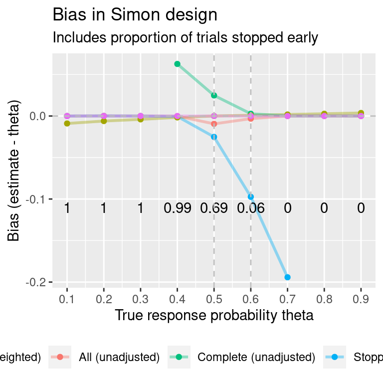
#>   theta MC error: bias MC error: SE
#> 1   0.1        0.00009      0.00007
#> 2   0.2        0.00012      0.00009
#> 3   0.3        0.00014      0.00010
#> 4   0.4        0.00015      0.00011
#> 5   0.5        0.00012      0.00009
#> 6   0.6        0.00012      0.00009
#> 7   0.7        0.00009      0.00007
#> 8   0.8        0.00008      0.00006
#> 9   0.9        0.00006      0.00004
Plot the same results, but removing the subsets “stopped early” or “stopped at N”:
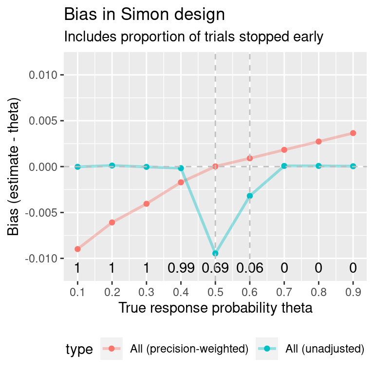
Simulate trials again, using values of p0 and p1 that are not close to 0.5
ADEMP
- Aim: Compare unconditional and precision-weighted bias in a Simon design (again)
- Data-generating mechanism:
- Binary outcome with a series of response rates (0.5, 0.9, 0.05)
- Type-I error-rate 0.05 when response rate p0=0.8 and power 0.90 when response rate p1=0.9
- Corresponding design: N=127, n1=44. Trial failure if number of responses less than or equal to 36 at interim or less than or equal to 108 at end.
- Estimand: response rate
- Method of analysis: point estimate, SE
- Performance measures: Conditional and precision-weighted bias
- Number of simulations: 1e5
all.designs2 <- clinfun::ph2simon(pu=0.8,
                                 pa=0.9,
                                 ep1=0.05,
                                 ep2=0.1,
                                 nmax=150)
# Choose optimal Simon design:
opt.index <- which.min(all.designs2$out[, "EN(p0)"])
simon.des2 <- all.designs2$out[opt.index, ]
Show results for response rates (0.10, 0.90, 0.05):
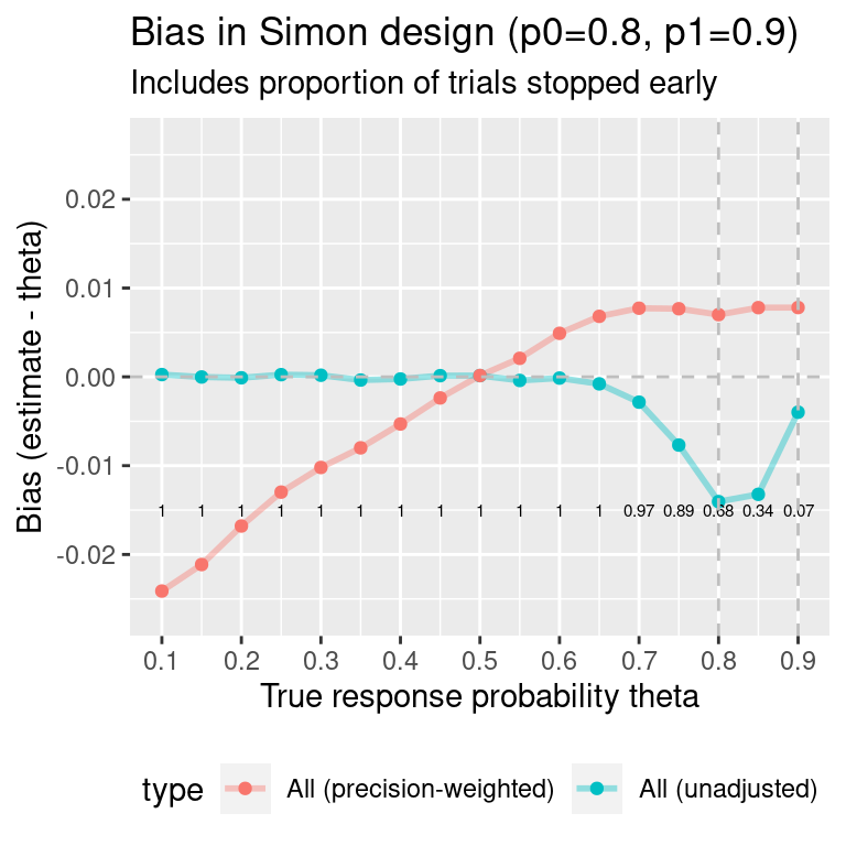
#>    theta MC error: bias MC error: SE
#> 1   0.10        0.00014      0.00010
#> 2   0.15        0.00017      0.00012
#> 3   0.20        0.00019      0.00013
#> 4   0.25        0.00021      0.00015
#> 5   0.30        0.00022      0.00016
#> 6   0.35        0.00023      0.00016
#> 7   0.40        0.00023      0.00017
#> 8   0.45        0.00024      0.00017
#> 9   0.50        0.00024      0.00017
#> 10  0.55        0.00024      0.00017
#> 11  0.60        0.00023      0.00016
#> 12  0.65        0.00022      0.00016
#> 13  0.70        0.00021      0.00015
#> 14  0.75        0.00018      0.00013
#> 15  0.80        0.00015      0.00011
#> 16  0.85        0.00014      0.00010
#> 17  0.90        0.00011      0.00008