Non-adaptive designs • pwb

library(pwb)
library(ggplot2)

Depending on the type of adaptation and the observed data, the progress of an adaptive design may not differ from a non-adaptive design. As such, it may be worthwhile to examine precision weighted bias in the context of non-adaptive designs. We simulate nsims=1e5 binary outcome single-stage designs with sample size N=100 for a series of response probabilities theta (0.1, 0.9, 0.1), then record the unadjusted and precision weighted bias:

# Simulate single-stage design:
nsims <- 1e5
N <- 100
theta.vec <- seq(0.1, 0.9, 0.1)
unadjusted <- pwbias <- numeric(length(theta.vec))
se.list <- vector("list", length(theta.vec))

for (i in 1:length(theta.vec)) {
  responses <- rbinom(nsims, N, theta.vec[i])
  theta.hat <- responses/N
  unadjusted[i] <- mean(theta.hat-theta.vec[i])
  se <- sqrt(theta.hat*(1-theta.hat)/N)
  pwbias[i] <- weighted.mean(x=theta.hat-theta.vec[i], w=1/se^2)
  se.list[[i]] <- se
}

dat <- data.frame(theta=rep(theta.vec, times=2),
                  bias=c(unadjusted, pwbias),
                  type=rep(c("unadjusted", "precision weighted"), each=length(theta.vec)))

se.df <- data.frame(se=unlist(se.list),
                    theta=rep(as.character(theta.vec), each=nsims))

#> Warning: Removed 2 rows containing missing values (`geom_line()`).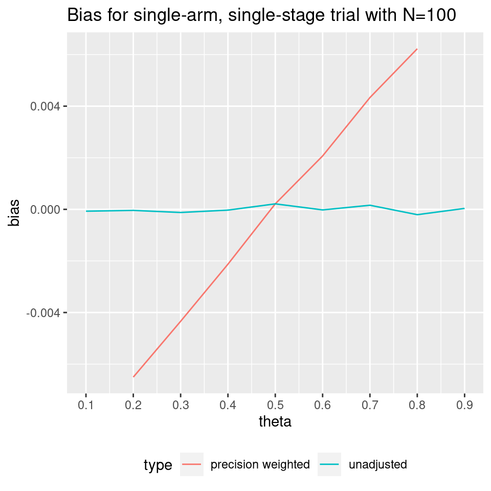

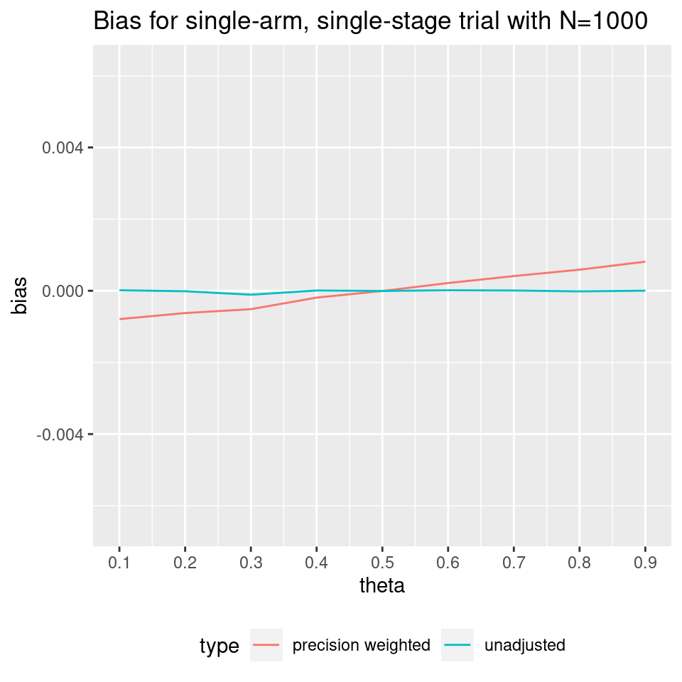
This effect decreases as N increases. For example, when N=1000:

Here is the distribution of standard errors for the N=100 data: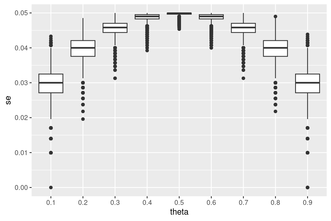

The farther theta is from 0.5, the greater the variation in SE. This increased variation means increased variation in weight, with more extreme (i.e. close to 0 or 1) values of theta hat receiving the most weight when calculating precision weighted bias. When theta is close to 0.5, there is low variation in SE, and weights will be similar (and then the weighted mean will be close to the mean).