GS
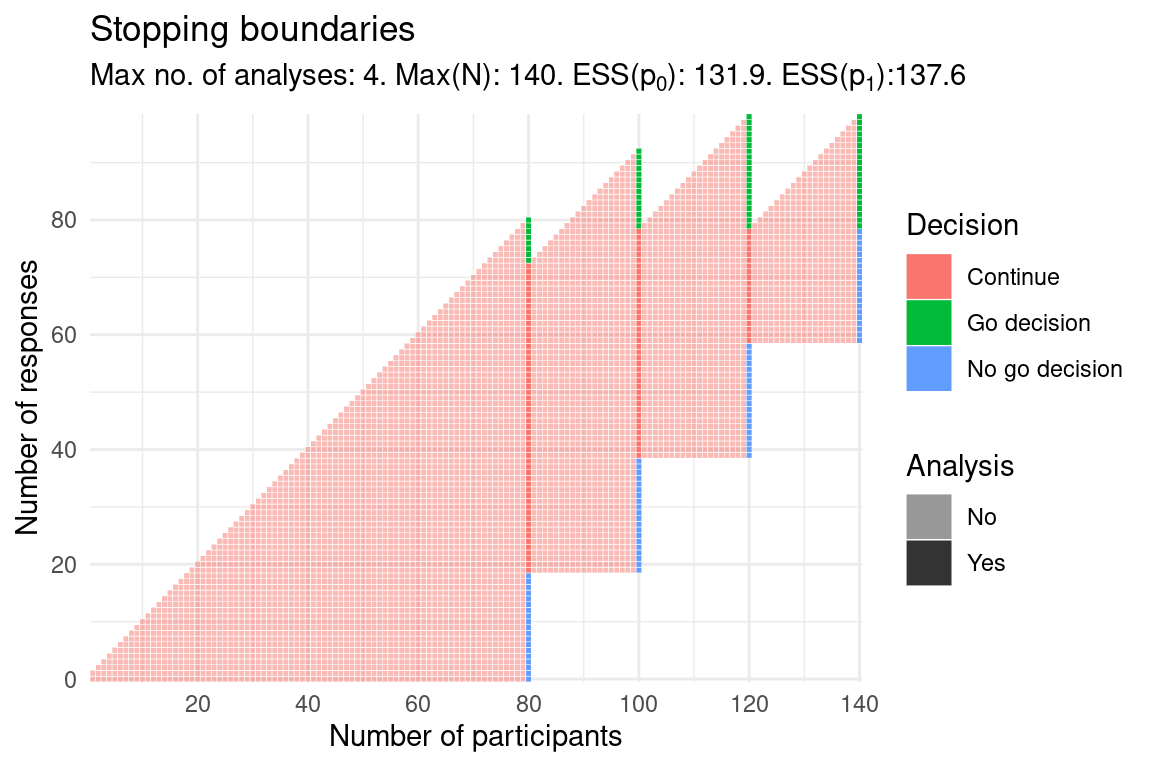
GS.RmdFind single-arm group sequential design with p0=0.5, p1=0.6, type-I error-rate 0.1, power 0.8, with stopping for both benefit and futility:
# Find bias for this design, for a single true response probability theta:
  nsims <- 1e5
  single.GS <- pwbGS(theta=0.5,
                     des=ad,
                     bounds=bounds$bounds.mat,
                     nsims=nsims)
  single.GS$ests[, 1:5]
#>                          nsims    bias mean.SE emp.SE theta
#> Stopped early            39311 -0.0452  0.0455 0.0276   0.5
#> Complete                 60689  0.0248  0.0421 0.0300   0.5
#> All                     100000 -0.0027  0.0435 0.0449   0.5
#> All (precision-weghted) 100000  0.0000  0.0433     NA   0.5
  round(single.GS$mc.error, 5)
#> [1] 0.00014 0.00010
How does bias compare when the true response probability is varied? Find results for a vector of true response probabilities:
theta.vec <- seq(0.2, 0.8, 0.1) # Vector of true response probabilities
summary.data <- raw.data <- vector("list", length(theta.vec))
stop.early.count <- rep(NA, length(theta.vec))
set.seed(53)
for(i in 1:length(theta.vec)){
one.run <- pwbGS(theta=theta.vec[i], des=ad, bounds=bounds$bounds.mat, nsims=nsims)
summary.data[[i]] <- one.run$ests
stop.early.count[i] <- one.run$ests["Stopped early", "nsims"]/nsims
}
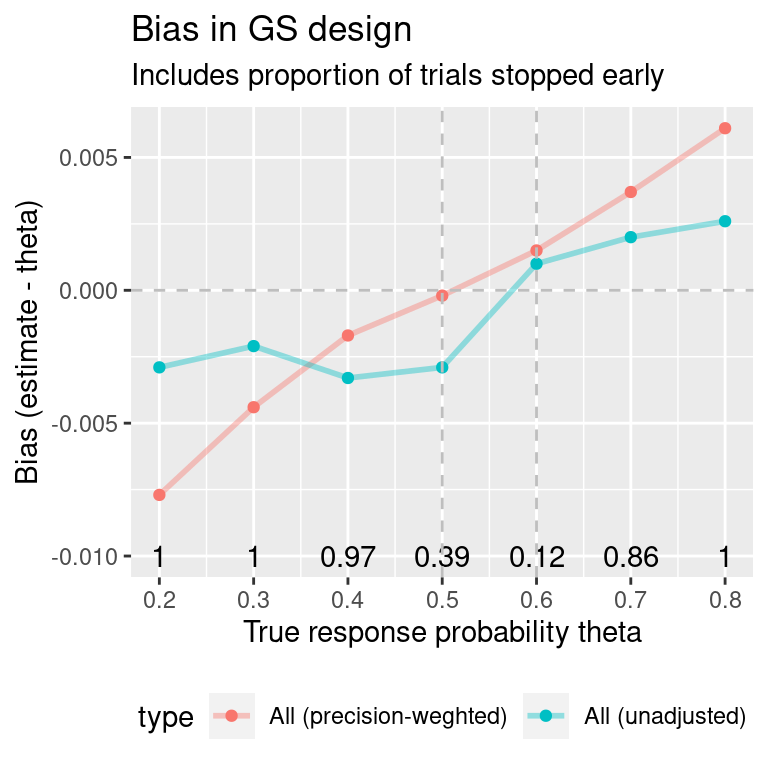
all.gs <- do.call(rbind, summary.data)Plot the results for all theta values:
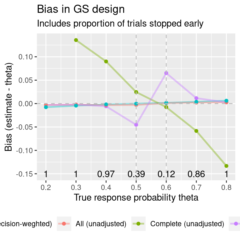
Plot the same results, but removing the subsets “stopped early” or
“stopped at N”: