Meta-Analysis on Postoperative Pneumonia • dcv

library(metafor)

Input data

dat <- escalc(measure="RR",
              ai=c(3,   5,  2,  0,  1),
              bi=c(32, 39, 43, 15, 24),
              ci=c(6,   7,  4,  1,  2),
              di=c(29, 35, 41, 14, 23),
              slab=c("Mahmoud et al, 2017",
                     "Li et al (Standard), 2020",
                     "Li et al (OLA), 2020",
                     "Ammar et al, 2021",
                     "Yao et al, 2020"))

Primary analysis: Paul-Mandel without Hartung-Knapp-Sidik-Jonkman (HKSJ) modification

pm <- rma(yi, vi, data=dat, method="PM") 
forest(pm,
       atransf=exp,
       at=log(c(0.01, 0.1, 0.5, 1, 4, 10)))

These results agree with the paper (Fig 2, top).

Sensitivity analysis

Sensitivity analysis 1: FE model

fe <- rma(yi, vi, data=dat, method="FE") 
forest(fe, 
       atransf=exp,
       at=log(c(0.01, 0.1, 0.5, 1, 4, 10)))

Note: The standard RE model without HKSJ modification is identical (not shown):

re <- rma(yi, vi, data=dat, method="REML")

Sensitivity analysis 2: Paule-Mandel with HKSJ modification

pmhk <- rma(yi, vi, data=dat, method="PM", test="knha") 
forest(pmhk,
       atransf=exp,
       at=log(c(0.01, 0.1, 0.5, 1, 4, 10)))

Sensitivity analysis 3: Odds ratios (Paule-Mandel without HKSJ modification)

dat.OR <- escalc(measure="OR",
              ai=c(3,   5,  2,  0,  1),
              bi=c(32, 39, 43, 15, 24),
              ci=c( 6,  7,  4,  1,  2),
              di=c(29, 35, 41, 14, 23),
              slab=c("Mahmoud et al, 2017",
                     "Li et al (Standard), 2020",
                     "Li et al (OLA), 2020",
                     "Ammar et al, 2021",
                     "Yao et al, 2020"))

Results are similar:

pm.OR <- rma(yi, vi, data=dat.OR, method="PM") 
forest(pm.OR,
       atransf=exp,
       at=log(c(0.01, 0.1, 0.5, 1, 4, 10)))

Sensitivity analysis 4: leave-one-out analysis

leave1 <- leave1out(pm)
forest.default(x=leave1$estimate, ci.lb=leave1$ci.lb, ci.ub=leave1$ci.ub,
               slab=paste("Omitting ", leave1$slab, sep=""),atransf=exp,
               at=log(c(0.15, 0.25, exp(pm$b),  1, 4)), xlim=log(c(0.01, 4.5)),
               refline=pm$b
              )
lines(x=log(c(1, 1)), y=c(0, 6))

The results of the leave-one-out sensitivity analysis agree with the paper (page 20, bottom, different order)

Funnel plot

funnel(pm, main="Standard Error")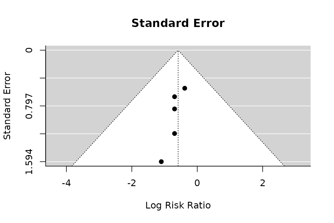

regtest(pm)
#> 
#> Regression Test for Funnel Plot Asymmetry
#> 
#> Model:     mixed-effects meta-regression model
#> Predictor: standard error
#> 
#> Test for Funnel Plot Asymmetry: z = -0.4407, p = 0.6594
#> Limit Estimate (as sei -> 0):   b = -0.1608 (CI: -2.1656, 1.8441)